Multi-Agent Reinforcement Learning (MARL) Engineering for Complex System Optimization: Building Autonomous Decision-Making Systems in Finance, Manufacturing, and Logistics
In systems where distributed decision-making entities interact, leading to complex optimization problems, traditional single-agent reinforcement learning or heuristic-based approaches face limitations. Multi-Agent Reinforcement Learning (MARL) is a key technology that enables dynamic and autonomous optimization of such complex systems, with the potential to create innovative business value ranging from financial portfolio management to production lines in smart factories and efficient resource allocation in logistics networks.
1. The Challenge / Context
Modern business environments are characterized by two features: complexity and interdependence. High-frequency trading in financial markets, dynamic production planning in manufacturing processes, and real-time route optimization in logistics networks—in all these areas, numerous independent elements interact and influence each other, determining the overall system performance. Traditional optimization techniques often rely on fixed environmental assumptions or centralized control models, making it difficult to effectively respond to unpredictable changes or the behavior of distributed decision-making entities. For example, in logistics, a delay in one vehicle can cause a domino effect across the entire supply chain, and in manufacturing, a malfunction of a specific machine can lead to bottlenecks throughout the production line. In such dynamic environments, making optimal decisions is often computationally impractical or lacks real-time capability. This is where Multi-Agent Reinforcement Learning (MARL) emerges as a powerful solution. The ability of each agent to learn autonomously by interacting with the environment, and to achieve goals cooperatively or competitively by considering the actions of other agents, becomes the key to solving the inherent complexity of complex systems.
2. Deep Dive: Multi-Agent Reinforcement Learning (MARL)
Multi-Agent Reinforcement Learning (MARL), as its name suggests, is a field of reinforcement learning where multiple "agents" simultaneously interact in the same environment to learn optimal policies. While single-agent reinforcement learning involves a single entity continuously interacting with the environment to learn how to maximize rewards, MARL fundamentally differs in that this "environment" includes the actions of other agents.
- Agents: Independent decision-making entities within the system. For example, in a financial system, each trading bot; in a manufacturing plant, each robotic arm or production facility; in a logistics system, each delivery vehicle can be an agent.
- Environment: The object with which all agents interact and are influenced by. This includes physical space, system state variables, and the actions of other agents.
- State, Action, Reward: Each agent observes the current state of the environment (which may be partially observed), selects an action within a defined action space. As a result of this action, the environment changes, and the agent receives a reward. Through this reward, the agent learns how much its actions contributed to achieving long-term goals.
- Policy: An agent's strategy for what action to take in a given state. The goal of MARL is to learn the optimal policy for each agent.
MARL is divided into various paradigms, but the most commonly applied to real-world complex systems is the Centralized Training, Decentralized Execution (CTDE) approach.
- Centralized Training: During the training phase, observation, action, and reward information from all agents are collected centrally to understand the overall system state and jointly optimize each agent's policy. This allows for effective learning of complex interactions and cooperative strategies among agents. For example, algorithms like QMIX and MADDPG fall into this category.
- Decentralized Execution: After training is complete, each agent makes decisions independently using only its learned policy, without centralized control. This ensures real-time performance and scalability, and offers the advantage of protecting the system from single points of failure such as communication delays or central server malfunctions.
CTDE is highly suitable for complex engineering problems because it allows for sufficient consideration of the impact of individual agent actions on the entire system during the learning phase, while maintaining high efficiency through independent decision-making in the actual operating environment.
3. Step-by-Step Guide / Implementation
Building a MARL-based autonomous decision-making system is much more complex than single-agent RL, requiring a deep understanding of the entire system and careful design. The following are the key steps.
Step 1: Problem Definition & Environment Modeling
The most crucial first step is to define the real-world problem within the MARL framework.
- Agent Identification: Clearly define the entities that need to act autonomously within the system. (e.g., each transport robot in a logistics center, each trading algorithm in a stock market)
- Environment State Definition: Define the information each agent can observe and the state of the entire environment. This must consider situations of Partial Observability. (e.g., robot's position, battery level, nearby item information, overall warehouse order status)
- Action Space Definition: Define the discrete or continuous actions each agent can perform. (e.g., robot's movement direction and speed, item pickup/drop)
- Environment Simulator Construction: Building a simulator that operates as similarly as possible to the real environment is essential. This efficiently generates the vast data needed for agent learning and allows for safe verification before deployment to the actual system.
# 예시: 물류 창고 로봇 환경 모델링 (Python-like pseudo-code)

class WarehouseEnv:
    def __init__(self, num_robots, grid_size, item_locations, delivery_points):
        self.num_robots = num_robots
        self.grid_size = grid_size
        self.item_locations = item_locations # 현재 물품 위치
        self.delivery_points = delivery_points # 배송 지점
        self.robot_positions = [...] # 각 로봇의 (x, y)
        self.robot_states = [...] # 각 로봇의 (배터리, 현재 운반 물품 ID)
        self.current_orders = [...] # 활성화된 주문 목록 (물품 ID, 목적지)
        self.timestep = 0

    def get_global_state(self):
        # 모든 에이전트가 볼 수 있는 전체 환경 상태 (중앙 학습 시 사용)
        return {
            "robot_positions": self.robot_positions,
            "robot_states": self.robot_states,
            "item_locations": self.item_locations,
            "current_orders": self.current_orders,
            "time": self.timestep
        }

    def get_agent_observation(self, agent_id):
        # 각 에이전트가 관측하는 부분적 상태
        return {
            "own_position": self.robot_positions[agent_id],
            "own_state": self.robot_states[agent_id],
            "nearby_robots": self._get_nearby_robot_info(agent_id),
            "nearby_items": self._get_nearby_item_info(agent_id),
            "assigned_order": self._get_assigned_order(agent_id)
        }

    def step(self, actions): # actions는 {agent_id: action} 딕셔너리
        rewards = {agent_id: 0 for agent_id in range(self.num_robots)}
        # 모든 에이전트의 행동을 한 번에 처리
        for agent_id, action in actions.items():
            # 행동에 따른 로봇 위치, 상태, 물품 위치 업데이트 로직 구현
            # ...
            # 개별 보상 계산
            rewards[agent_id] = self._calculate_individual_reward(agent_id, action)

        # 전체 환경 업데이트 (시간 경과, 새로운 주문 발생 등)
        self.timestep += 1
        global_reward = self._calculate_global_reward(rewards) # 전체 시스템 목표에 대한 보상
        done = self._check_termination_condition()
        return self.get_global_state(), rewards, done, {}

    def reset(self):
        # 환경 초기화
        # ...
        return self.get_global_state()

    # 내부 헬퍼 함수들 (예: 충돌 감지, 최단 경로 계산 등)
    # ...
Step 2: MARL Architecture & Algorithm Selection
Select an appropriate MARL architecture and algorithm based on the problem's characteristics and the relationships between agents (cooperative, competitive, or mixed).
- CTDE (Centralized Training, Decentralized Execution): Suitable for most complex system problems. Particularly effective when clear cooperation or complex coordination between agents is required. QMIX, MADDPG, and COMA are representative examples.
- Independent Learners: Each agent treats other agents as part of the environment and learns independently. This approach is simple to implement but can suffer from learning instability due to the non-stationarity problem.
-
Architecture Selection Guide:
- QMIX: A value-based algorithm that estimates the overall system's Q-value by decomposably estimating individual agent Q-values to learn cooperative behaviors. Advantageous for discrete action spaces.
- MADDPG (Multi-Agent Deep Deterministic Policy Gradient): An Actor-Critic-based algorithm suitable for continuous action spaces and applicable to both competitive and cooperative environments.
- COMA (Counterfactual Multi-Agent Policy Gradients): A policy gradient-based algorithm where the critic uses a 'counterfactual' baseline, removing the actions of other agents, to clearly evaluate each agent's contribution.
Step 3: Reward Function Design
The success of MARL heavily depends on reward function design. It is much more complex than for single agents and requires considering the following:
- Global Reward: Reward for achieving the overall system goal. (e.g., reducing total order processing time in a logistics warehouse, increasing total production volume on a production line)
- Individual Reward: Reward for each agent's direct actions. (e.g., reward when a robot successfully picks up/delivers an item)
- Credit Assignment Problem: The difficulty in determining how much each agent contributed to a global reward when it is given. CTDE architectures and specific algorithms (e.g., COMA) help address this.
- Addressing Sparse Rewards: When rewards are infrequent, shaping techniques or Auxiliary Rewards can be used to accelerate learning. For example, giving a reward as an agent gets closer to an item.
- Penalty Design: Clearly define penalties for undesirable behaviors such as collisions, delays, or resource waste.
Step 4: Building the Training Pipeline & Training
Implement the training pipeline based on the constructed simulator and selected algorithm.
- Library Selection: Utilize MARL-specific libraries such as PyMARL, RLlib, or PettingZoo to reduce implementation complexity.
- Neural Network Architecture Definition: Design neural networks (e.g., MLP, CNN, RNN) to approximate each agent's policy and value function. If there are many agents or they have similar roles, parameter sharing can improve learning efficiency.
- Experience Replay Buffer: Store (state, action, reward, next state) tuples experienced by agents and sample them randomly to improve learning stability.
- Optimization: Update neural network parameters using optimization algorithms like Adam or RMSprop.
- Hyperparameter Tuning: Carefully tune various hyperparameters such as learning rate, discount factor, exploration policy (epsilon-greedy), and buffer size.
# 예시: PyMARL (QMIX) 기반 학습 루프 (pseudo-code)

import torch
import numpy as np
from smac.env import StarCraft2Env # 예시 환경 (실제로는 WarehouseEnv 등 사용)
from qmix_agent import QMIX

# 1. 환경 초기화
env = WarehouseEnv(num_robots=5, ...) # Step 1에서 정의한 환경
state_dim = env.get_global_state_dim()
obs_dim = env.get_agent_observation_dim()
n_actions = env.get_agent_action_space_size()
n_agents = env.num_robots

# 2. QMIX 에이전트 초기화
agent = QMIX(state_dim, obs_dim, n_actions, n_agents, device='cuda' if torch.cuda.is_available() else 'cpu')

# 3. 학습 파이프라인
num_episodes = 10000
max_timesteps_per_episode = 200

for episode in range(num_episodes):
    env_state = env.reset()
    episode_reward = 0
    done = False

    # 에피소드 데이터 수집 버퍼
    episode_data = []

    for t in range(max_timesteps_per_episode):
        # 각 에이전트의 관측 기반으로 행동 결정 (exploration 포함)
        agent_observations = [env.get_agent_observation(i) for i in range(n_agents)]
        actions = agent.select_actions(agent_observations) # QMIX 내부에서 epsilon-greedy 적용

        # 환경에 행동 적용
        next_env_state, rewards_dict, done, _ = env.step(actions)

        # QMIX는 보통 전역 보상을 사용하거나, 개별 보상으로부터 전역 보상을 계산
        global_reward = sum(rewards_dict.values())
        episode_reward += global_reward

        # 경험 버퍼에 저장 (CTDE이므로 모든 에이전트의 정보와 전역 보상 저장)
        episode_data.append({
            "obs": agent_observations,
            "state": env_state,
            "actions": actions,
            "reward": global_reward, # 전역 보상
            "next_obs": [env.get_agent_observation(i) for i in range(n_agents)],
            "next_state": next_env_state,
            "done": done
        })

        env_state = next_env_state

        if done:
            break

    # 에피소드 종료 후 일괄 학습 (배치 학습)
    agent.add_episode_to_buffer(episode_data)
    if agent.can_train(): # 버퍼에 충분한 데이터가 쌓였을 때
        agent.train()

    if episode % 100 == 0:
        print(f"Episode: {episode}, Total Reward: {episode_reward}")

# 학습 완료 후 모델 저장
agent.save_model("qmix_warehouse_model.pth")
Step 5: Deployment & Monitoring Strategy
Applying the learned policies to real systems and operating them stably is another critical challenge.
- Minimizing Sim-to-Real Gap: The simulation environment may differ from the real environment. Techniques such as Domain Randomization, Domain Adaptation, and adjusting the simulation using real data should be employed to reduce this gap.
- Ensuring Safety and Robustness: Agent behavior in unpredictable situations must be verified, and safety constraints should be integrated into the policy or external Safety Filters introduced.
- Phased Rollout: Rather than applying to the entire system at once, it is advisable to first apply to a limited area or specific agents to verify effectiveness and stability, then gradually expand.
- Performance Monitoring: After deployment, real-time monitoring of agent behavior, key system indicators (KPIs), and reward values is necessary to detect anomalies and perform retraining or manual intervention if needed. If model performance degrades, establishing an automated retraining pipeline (MLOps) can be considered.
4. Real-world Use Case / Example
Production Line Optimization in Smart Factories
Traditional smart factory production lines are operated through pre-defined rules or optimization algorithms (e.g., linear programming) via MES (Manufacturing Execution System) or ERP (Enterprise Resource Planning) systems. However, production lines are dynamic environments. Unpredictable variables such as machine breakdowns, sudden order changes, raw material supply instability, and changes in worker skill levels occur in real-time. In such situations, fixed rules can lead to bottlenecks, increased idle time, and reduced productivity.MARL offers an innovative solution to these problems. Each major piece of equipment on the production line (robotic arm, CNC machine, inspection equipment, AGV (Autonomous Guided Vehicle)) is modeled as an agent.
- Agents: Each work station, transport AGV, quality inspection robot.
- Observation: Own work status, next task queue, status of adjacent agents, overall production line goal achievement rate, current order information.
- Action: Start/stop work, transfer items to the next process, change priority, remain idle, adjust speed.
- Reward: Faster task processing by individual agents (individual reward), along with increased total production volume, minimized bottlenecks, and reduced defect rates for the entire production line (global reward).
How MARL Works: Using a CTDE approach, during the training phase, the states and actions of all agents are integrated centrally to understand the complex dynamics of the entire production line and learn optimal cooperative strategies. For example, if one robotic arm finishes processing a workpiece, but the robot in the next process is not yet ready, this robotic arm can learn a strategy to process other lower-priority tasks first, or wait for a moment to avoid exacerbating the bottleneck in the next process. The learned policies are deployed to each piece of equipment, enabling autonomous optimal decision-making in response to real-time changes in the production environment.
Personal Opinion: The biggest challenge in this field is the "realism of the simulation environment." Actual factory environments include numerous variables (sensor noise, subtle machine malfunctions, network delays) that are difficult to perfectly reproduce in simulation. Therefore, it is essential to actively utilize techniques like Domain Randomization to make the simulator robust to various realistic variations, and to build an MLOps pipeline that continuously fine-tunes the model through a data feedback loop with the actual system. Beyond merely understanding algorithms, tangible results can only be achieved when domain knowledge and system engineering capabilities are combined.
5. Pros & Cons / Critical Analysis
-
Pros:
- Handling Complex Interactions: Can autonomously learn optimal cooperative/competitive strategies in systems where numerous agents interact complexly.
- Dynamic Environment Adaptation: More flexibly responds to unpredictable changes or uncertainties than traditional optimization techniques, adjusting decision-making policies in real-time.
- Emergent Behavior: Can learn unexpected strategies or behavior patterns that are beneficial to the entire system, even if not explicitly programmed.
- Robust to Partial Observability: Can make effective decisions with limited information, even if each agent does not know the entire system state.
- Scalability: Provides an architecture that can be relatively easily scaled even when the number of agents increases or system complexity grows (especially when applying parameter sharing techniques).
-
Cons:
- High Computational Cost and Training Time: Due to multiple agents and complex environments, training requires an enormous amount of computing resources and time.
- Difficulty in Reward Function Design: It is very challenging to accurately evaluate the contribution of each agent and design a reward function that harmoniously reflects both overall system goals and individual agent goals (Credit Assignment Problem).
- Learning Stability and Convergence Issues: As multiple agents learn simultaneously, the environment can become non-stationary, leading to unstable learning or failure to converge.
- Sim-to-Real Gap: Policies learned in a simulation environment may not perform as expected in the real environment. Reducing the gap between reality and simulation is a key challenge.
- Lack of Interpretability: Deep learning-based MARL models operate as black boxes, making it difficult to explain why a particular decision was made. This can pose challenges for regulatory compliance or problem-solving.
6. FAQ
-
Q: What is the biggest difference between MARL and traditional optimization techniques (e.g., linear programming, genetic algorithms)?
A: The biggest difference is dynamic environment adaptability and autonomy. Traditional optimization techniques are generally based on fixed models or predefined rules and struggle to adapt to environmental changes in real-time. In contrast, MARL agents learn by interacting with the environment, autonomously finding and evolving optimal policies even in unpredictable changes. MARL is more powerful in systems with complex interactions and high uncertainty. -
Q: What MARL frameworks or libraries do you recommend?
A: If you are just starting, I recommend RLlib (Ray RLLib). It supports various single and multi-agent RL algorithms and facilitates building distributed learning environments. Also, PyMARL is specialized in implementing CTDE-based algorithms (QMIX, MADDPG, etc.) and has many integration examples with the StarCraft II environment, making it good for research. For simple multi-agent environment implementation and testing, PettingZoo is also useful. -
Q: What is the biggest challenge when applying MARL to real systems?
A: The biggest challenges are "building a reliable simulation environment" and "reward function design." It is difficult to perfectly reflect the complexity and noise of real systems in a simulator, which can lead to learned policies not working correctly in reality (Sim-to-Real Gap). Additionally, accurately and delicately designing a reward function that encourages cooperation or competition among agents and achieves overall system goals requires a high level of domain knowledge and experience.
7. Conclusion
Multi-Agent Reinforcement Learning (MARL) is more than just a technological advancement in optimizing complex systems like finance, manufacturing, and logistics; it is a field with the potential to transform the operating paradigm of systems themselves. This signifies an era where optimization is no longer isolated to single agents, but rather numerous intelligent agents cooperate and compete, autonomously evolving towards the goals of the entire system. Of course, there are many challenges to overcome, such as high computational costs, the difficulty of reward function design, and the gap between simulation and reality. However, by overcoming these difficulties, we will be able to build autonomous decision-making systems with levels of efficiency and flexibility previously unimaginable.
<